---
title: "Technical Report"
jupyter: python3
---
## Introduction
This project analyzes Utah residential housing listings in several cities in Salt Lake County and Utah counties to explore, build, and evaluate predictive models for house `price`.
The motivation for this project is to provide data-driven guidance for buyers, sellers, and local planners by identifying key predictors of sale price and producing models that balance predictive accuracy and interpretability.
Some key goals of this project were (1) to produce clear exploratory analyses that reveal relationships between `price` and common housing attributes; (2) to fit defensible regression models (i.e. best-subsets by AIC and a LASSO-regularized model) and compare them using cross-validated PMSE; and (3) to document reproducible code and a small interactive Streamlit app for sharing results.
## Data Source and Methodology
1. Data acquisition:
- Raw listings were collected from UtahRealEstate.com with the repository's scraping scripts. The primary ingestion function used in this report is `data_no_scape()` which returns the raw DataFrame used for downstream processing.
2. Cleaning pipeline:
- The cleaning pipeline performs the following steps: removing obvious duplicates, dropping invalid or malformed entries, and standardizing numeric columns (e.g. beds, baths, sqft). For purposes of analysis, we dropped the original `address` and `mls` fields.
3. Analysis workflow:
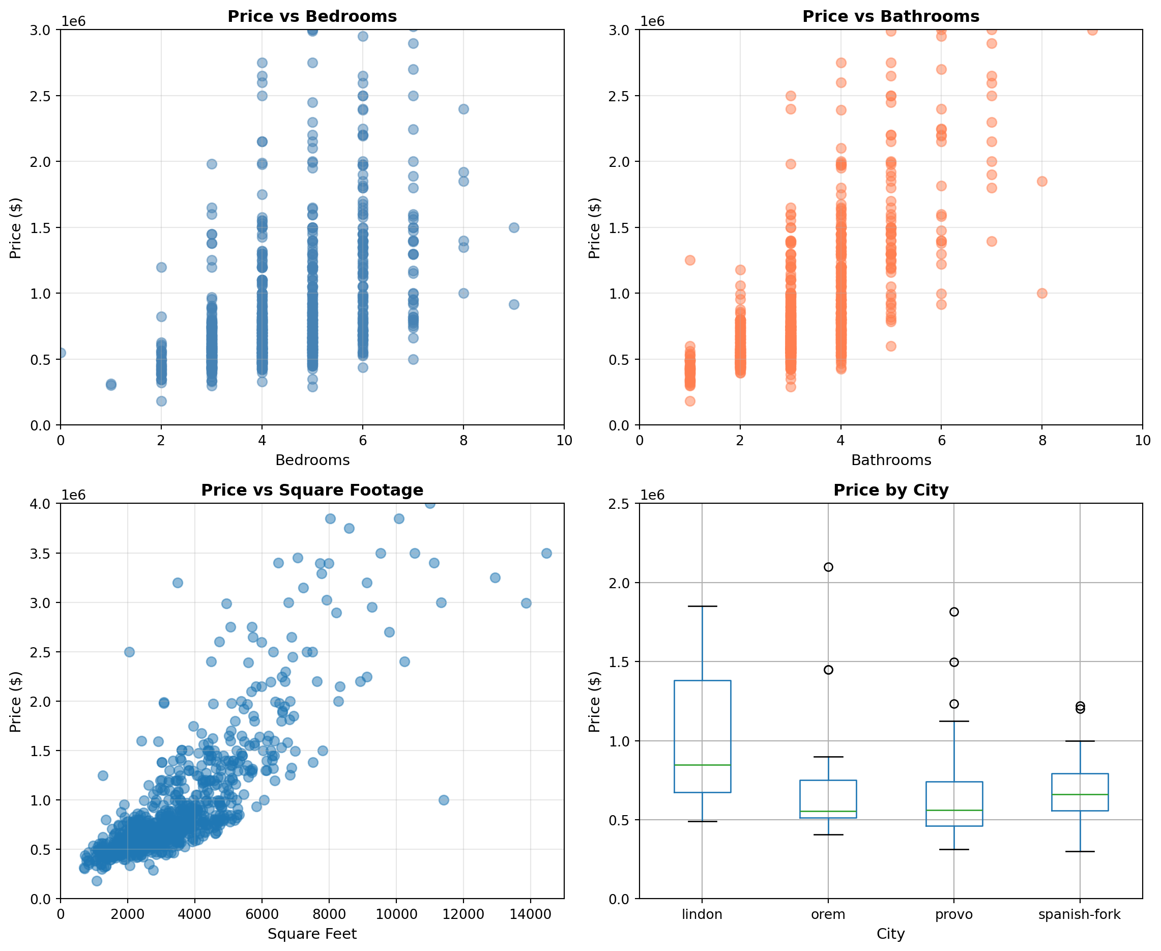
- Exploratory data analysis involved visual checks (scatterplots and boxplots) to inspect relationships between `price` and candidate predictors and to assess outliers and heterogeneity across selected cities.
- Model selection involved exhaustive best-subsets regression evaluated by AIC to identify an interpretable model, and LASSO (with cross-validated penalty) to perform automated variable selection and shrinkage. Models were fit with `statsmodels` and model summaries were constructed with `patsy`.
- Model assessment: 5-fold cross-validation is used to estimate the predictive mean squared error (PMSE) for competing models.
4. Tooling and reproducibility:
- Primary libraries: `pandas`, `numpy`, `matplotlib`, `seaborn`, `statsmodels`, `patsy`, `scikit-learn`.
- Project environment and packaging: see `pyproject.toml`
## EDA
```{python}
#| include: false
import pandas as pd
from utah_housing_stat386.cleaning import data_no_scape, cleaned_static_data, clean_housing_data, remove_duplicates, remove_invalid_entries
import re
df_raw = data_no_scape()
df_clean2 = clean_housing_data(df_raw)
df_clean2 = remove_duplicates(df_clean2)
df_clean2 = remove_invalid_entries(df_clean2)
df = df_clean2.copy()
address_list = df['address'].tolist()
pattern = r"UT \d{5}"
zipcode_list = []
for address in address_list:
zipcode_list.append(re.search(pattern, address).group()[3:])
df['zipcode'] = zipcode_list
df = df.drop(columns=['address', 'mls', 'zipcode'])
```
```{python}
import matplotlib.pyplot as plt
import numpy as np

# Create a 2x2 figure with 4 subplots
fig, axes = plt.subplots(2, 2, figsize=(12, 10))
fig.suptitle('EDA: Price vs Selected Variables', fontsize=16, fontweight='bold')

# Plot 1 (top-left): Scatterplot - price vs bedrooms (or sqft, year_built, etc.)
axes[0, 0].scatter(df['beds'], df['price'], alpha=0.5, s=50, color='steelblue')
axes[0, 0].set_xlabel('Bedrooms', fontsize=11)
axes[0, 0].set_ylabel('Price ($)', fontsize=11)
axes[0, 0].set_title('Price vs Bedrooms', fontweight='bold')
axes[0, 0].grid(True, alpha=0.3)
axes[0, 0].set_xlim(0, 10)
axes[0, 0].set_ylim(0, 3_000_000)

# Plot 2 (top-right): Scatterplot - price vs bathrooms (or sqft, lot_size, etc.)
axes[0, 1].scatter(df['baths'], df['price'], alpha=0.5, s=50, color='coral')
axes[0, 1].set_xlabel('Bathrooms', fontsize=11)
axes[0, 1].set_ylabel('Price ($)', fontsize=11)
axes[0, 1].set_title('Price vs Bathrooms', fontweight='bold')
axes[0, 1].grid(True, alpha=0.3)
axes[0, 1].set_xlim(0, 10)
axes[0, 1].set_ylim(0, 3_000_000)

# Plot 3 (bottom-left): Boxplot - price by garage (categorical)
axes[1, 0].scatter(df['sqft'], df['price'], alpha=0.5, s=50)
axes[1, 0].set_xlabel('Square Feet', fontsize=11)
axes[1, 0].set_ylabel('Price ($)', fontsize=11)
axes[1, 0].set_title('Price vs Square Footage', fontweight='bold')
axes[1, 0].grid(True, alpha=0.3)
axes[1, 0].set_xlim(0, 15_000)
axes[1, 0].set_ylim(0, 4_000_000)

# Plot 4 (bottom-right): Boxplot - price by city (categorical)
sub_df = df[df['city'].isin(['lindon', 'orem', 'provo', 'spanish-fork'])]
sub_df.boxplot(column='price', by='city', ax=axes[1, 1])
axes[1, 1].set_xlabel('City', fontsize=11)
axes[1, 1].set_ylabel('Price ($)', fontsize=11)
axes[1, 1].set_title('Price by City', fontweight='bold')
axes[1, 1].get_figure().suptitle('')  # remove automatic title from boxplot
axes[1, 1].set_ylim(0, 2_500_000)

plt.tight_layout()
plt.show()
```
## Link to Streamlit App
[Link to Streamlit app](https://stat386finalproject-seth-carson-4.streamlit.app/)
## Analysis
```{python}
#| message: false
#| warning: false
# Import necessary modules
import itertools
import statsmodels.formula.api as smf
from patsy import dmatrices
from sklearn.model_selection import KFold
from sklearn.linear_model import LinearRegression, LassoCV, Lasso
from sklearn.preprocessing import StandardScaler
from sklearn.pipeline import Pipeline
from sklearn.metrics import mean_squared_error

# -----------------------------
# Treat ONLY city and zipcode as categorical
# -----------------------------
cat_vars = ['city', 'zipcode']
for c in cat_vars:
    if c in df.columns:
        df[c] = df[c].astype('category')

# Candidate predictors
candidates = [c for c in df.columns if c != 'price']

# -----------------------------
# Best subsets selection via AIC
# -----------------------------
best_aic = np.inf
best_formula = None
best_model = None

for k in range(1, len(candidates) + 1):
    for subset in itertools.combinations(candidates, k):
        terms = [f"C({v})" if v in cat_vars else v for v in subset]
        formula = "price ~ " + " + ".join(terms)
        try:
            model = smf.ols(formula, data=df).fit()
            if model.aic < best_aic:
                best_aic = model.aic
                best_formula = formula
                best_model = model
        except Exception:
            continue

print("\n==============================")
print("BEST SUBSETS (AIC) MODEL")
print("==============================")
print("Best AIC:", best_aic)
print("Best formula:", best_formula)
print(best_model.summary())

# -----------------------------
# CV PMSE for Best-AIC model
# -----------------------------
y_aic, X_aic = dmatrices(best_formula, data=df, return_type='dataframe')
y_aic = np.ravel(y_aic)

kf = KFold(n_splits=5, shuffle=True, random_state=1)
mses_aic = []

for tr, te in kf.split(X_aic):
    lr = LinearRegression(fit_intercept=False)
    lr.fit(X_aic.iloc[tr], y_aic[tr])
    preds = lr.predict(X_aic.iloc[te])
    mses_aic.append(mean_squared_error(y_aic[te], preds))

pmse_aic = np.mean(mses_aic)

# -----------------------------
# LASSO (lambda = 1 SE rule)
# -----------------------------
# Build full design matrix with dummies
full_formula = "price ~ " + " + ".join(
    [f"C({v})" if v in cat_vars else v for v in candidates]
)

y_lasso, X_lasso = dmatrices(full_formula, data=df, return_type='dataframe')
y_lasso = np.ravel(y_lasso)

# LASSO with standardization
lasso_cv = Pipeline([
    ("scaler", StandardScaler()),
    ("lasso", LassoCV(cv=5, random_state=1))
])

lasso_cv.fit(X_lasso, y_lasso)

# Lambda_1se
mse_path = lasso_cv.named_steps["lasso"].mse_path_.mean(axis=1)
mse_std = lasso_cv.named_steps["lasso"].mse_path_.std(axis=1)
idx_min = np.argmin(mse_path)
mse_1se = mse_path[idx_min] + mse_std[idx_min]
idx_1se = np.where(mse_path <= mse_1se)[0][-1]

alpha_1se = lasso_cv.named_steps["lasso"].alphas_[idx_1se]

# Fit LASSO at lambda_1se
lasso_1se = Pipeline([
    ("scaler", StandardScaler()),
    ("lasso", Lasso(alpha=alpha_1se))
])

lasso_1se.fit(X_lasso, y_lasso)

# Selected variables
coef = lasso_1se.named_steps["lasso"].coef_
selected = X_lasso.columns[coef != 0]

print("\n==============================")
print("LASSO SELECTED VARIABLES (λ_1se)")
print("==============================")
print(list(selected))

# -----------------------------
# Refit OLS using LASSO-selected variables (FIXED)
# -----------------------------

selected_cols = X_lasso.columns[coef != 0]

# Recover original variable names
selected_vars = set()

for col in selected_cols:
    if col.startswith("C("):
        # categorical: extract variable name inside C(...)
        var = col.split("[")[0]          # C(city)
        var = var.replace("C(", "").replace(")", "")
        selected_vars.add(f"C({var})")
    else:
        selected_vars.add(col)

selected_vars = sorted(selected_vars)

print("\nVariables used in LASSO refit:")
print(selected_vars)

lasso_formula = "price ~ " + " + ".join(selected_vars)
lasso_refit = smf.ols(lasso_formula, data=df).fit()

print("\n==============================")
print("OLS REFIT USING LASSO VARIABLES")
print("==============================")
print(lasso_refit.summary())

# -----------------------------
# CV PMSE for LASSO-selected model
# -----------------------------
y_lasso2, X_lasso2 = dmatrices(lasso_formula, data=df, return_type='dataframe')
y_lasso2 = np.ravel(y_lasso2)

mses_lasso = []
for tr, te in kf.split(X_lasso2):
    lr = LinearRegression(fit_intercept=False)
    lr.fit(X_lasso2.iloc[tr], y_lasso2[tr])
    preds = lr.predict(X_lasso2.iloc[te])
    mses_lasso.append(mean_squared_error(y_lasso2[te], preds))

pmse_lasso = np.mean(mses_lasso)

# -----------------------------
# Final comparison
# -----------------------------
print("\n==============================")
print("CROSS-VALIDATED PMSE COMPARISON")
print("==============================")
print(f"Best Subsets (AIC) PMSE : {pmse_aic:.3f}")
print(f"LASSO (1SE) PMSE        : {pmse_lasso:.3f}")
```
## Conclusion
The report compares two model-building strategies: exhaustive best-subsets selection using AIC and LASSO (with the 1-SE rule). Fitted model summaries are generated through `statsmodels`, and the models are evaluated using 5-fold cross-validated PMSE. The best‐subsets AIC procedure selected a parsimonious model containing only five structural predictors—beds, baths, square footage, year built, and lot size—yielding an ($R^2$) of 0.577 and the lowest AIC (30231.2) among all candidate models. All included predictors are statistically significant at the $\alpha=0.05$ level, with square footage and lot size positively associated with price, while the negative coefficient on beds likely reflects multicollinearity with square footage. This model emphasizes interpretability and achieves strong explanatory power with relatively few parameters.
In contrast, the LASSO model using the one–standard‐error rule selected a much richer specification that included the same core structural variables, added garage size, and incorporated city as a categorical factor, resulting in 26 fitted coefficients in the refit OLS model. This model achieved a slightly higher in‐sample fit ($R^2 = 0.593$), suggesting that location effects explain additional variation in housing prices beyond physical characteristics. However, many individual city coefficients are not statistically significant, indicating that while location matters collectively, its contribution is diffuse across levels rather than driven by a small number of dominant cities.
When comparing predictive performance via cross‐validation, the best‐subsets AIC model slightly outperformed the LASSO‐selected model, with a lower PMSE ($2.13 \times 10^{12}$ vs. $2.22 \times 10^{12}$). This suggests that the additional complexity introduced by the LASSO model does not translate into improved out‐of‐sample prediction. Overall, the results highlight a classic bias–variance tradeoff: the LASSO model captures more structure through location effects but incurs higher variance, while the simpler AIC‐selected model provides comparable and slightly superior—predictive accuracy with greater interpretability.
There are several limitations to consider. The scraped dataset may suffer from selection bias, as online listings do not represent all transactions, and measurement errors could exist in features such as square footage or number of bedrooms. Additionally, some predictors are coarse (e.g. `city`) and may obscure spatial heterogeneity. Residual heteroscedasticity and nonlinearity are also possible, suggesting that transforming the price variable (e.g., using $\log(\texttt{price})$) or applying robust, heteroscedasticity-consistent standard errors may be appropriate.
Future work could involve incorporating additional predictors such as year built, lot size, and proximity to amenities, or exploring spatial models that explicitly account for location dependence. Alternative loss functions like MAE could be evaluated, and tree-based ensemble methods such as random forests or gradient boosting could be applied, with comparisons of their calibrated uncertainty against linear models. Finally, the best-performing model could potentially be packaged and deployed via an endpoint or dashboard, enabling users to query price predictions based on property attributes.
From a practical standpoint, the results suggest that a sizeable portion of the information needed to predict home prices comes from a small set of basic property features, especially square footage, lot size, and overall layout. It was observed tha adding many location indicators increases model complexity without meaningfully improving predictive accuracy. For real-world use, such as quick price estimates, reporting, or decision support, the simpler AIC-selected model is likely the better choice: it is easier to explain, easier to maintain, and performs just as well (or slightly better) on new data. More complex models may still be useful for deeper analysis of neighborhood effects.